Variant transforms
In addition to the basic 1, 2 and 3 dimensional DT-CWT, this library also supports a selection of variant transforms.
Rotational symmetry modified wavelet transform
For some applications, one may prefer the subband responses to be more rotationally similar.
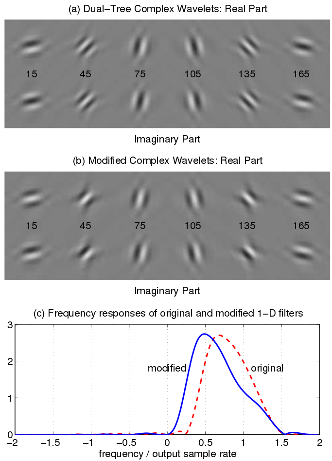
In the original 2-D DTCWT, the 45 and 135 degree subbands have passbands whose centre frequencies are somewhat further from the origin than those of the other four subbands. This results from the combination of two highpass 1-D wavelet filters to produce 2-D wavelets. The remaining subbands combine highpass and lowpass 1-D filters, and hence their centre frequencies are a factor of approximately sqrt(1.8) closer to the origin of the frequency plane.
The dtwavexfm2b() function employs an alternative bandpass 1-D filter in place of the highpass filter for the appropriate subbands. The image below illustrates the relevant differences in impulse and frequency responses[1].
Usage is very similar to the standard 2-D transform function, but the only supported parameters are ‘near_sym_b_bp’, ‘qshift_b_bp’. These arguments are optional, but it is best practice to include them so that your intentions are clear (and because it is easier for others to spot than the difference between 2() and 2b().
Yl, Yh = dtcwt.dtwavexfm2b(image, tfmlevel, 'near_sym_b_bp', 'qshift_b_bp')
While the Hilbert transform property of the DTCWT is preserved, perfect reconstruction is lost. However, in applications such as machine vision, where all subsequent operations on the image take place in the transform domain, this is of relatively minor importance.
For full details, refer to:
[1] N. G. Kingsbury. Rotation-invariant local feature matching with complex wavelets. In Proc. European Conference on Signal Processing (EUSIPCO), pages 901–904, 2006. 2, 18, 21
Example
Working on the Lena image, the standard 2-D DTCWT achieves perfect reconstruction:
# Perform the standard 2-D DTCWT
Yl, Yh = dtcwt.dtwavexfm2(image, tfmlevel, 'near_sym_b', 'qshift_b')

# Perform the inverse transform
Z = dtcwt.dtwaveifm2(Yl, Yh, biort='near_sym_b', qshift='qshift_b')

# Show the error
imshow(Z-image, cmap=cm.gray)
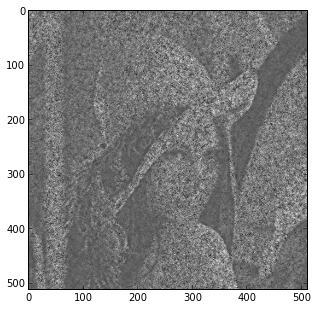
The error signal appears to be just noise, which we can attribute to floating-point precision.
Using the modified wavelets yields the following result:
# Perform the symmetry-modified 2-D DTCWT
Yl, Yh = dtcwt.dtwavexfm2b(image, tfmlevel, 'near_sym_b_bp', 'qshift_b_bp')

# Perform the inverse transform
Z = dtcwt.dtwaveifm2b(Yl, Yh, biort='near_sym_b_bp', qshift='qshift_b_bp')

# Show the error
imshow(Z-image, cmap=cm.gray)
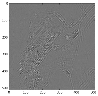
As we would expect, the error is more significant, but only near 45 and 135 degree edge features.