Getting Started¶

This section will guide you through using the dtcwt library. Once installed, you are most likely to use one of these functions:

dtcwt.dtwavexfm() – 1D DT-CWT transform.
dtcwt.dtwaveifm() – Inverse 1D DT-CWT transform.
dtcwt.dtwavexfm2() – 2D DT-CWT transform.
dtcwt.dtwaveifm2() – Inverse 2D DT-CWT transform.
dtcwt.dtwavexfm3() – 3D DT-CWT transform.
dtcwt.dtwaveifm3() – Inverse 3D DT-CWT transform.

See API Reference for full details on how to call these functions. We shall present some simple usage below.

Installation¶

The easiest way to install dtcwt is via easy_install or pip:

$ pip install dtcwt

If you want to check out the latest in-development version, look at the project’s GitHub page. Once checked out, installation is based on setuptools and follows the usual conventions for a Python project:

$ python setup.py install

(Although the develop command may be more useful if you intend to perform any significant modification to the library.) A test suite is provided so that you may verify the code works on your system:

$ python setup.py nosetests

This will also write test-coverage information to the cover/ directory.

Building the documentation¶

There is a pre-built version of this documentation available online and you can build your own copy via the Sphinx documentation system:

$ python setup.py build_sphinx

Compiled documentation may be found in build/docs/html/.

1D transform¶

This example generates two 1D random walks and demonstrates reconstructing them using the forward and inverse 1D transforms. Note that dtcwt.dtwavexfm() and dtcwt.dtwaveifm() will transform columns of an input array independently:

import numpy as np
from matplotlib.pyplot import *

# Generate a 300x2 array of a random walk
vecs = np.cumsum(np.random.rand(300,2) - 0.5, 0)

# Show input
figure(1)
plot(vecs)
title('Input')

import dtcwt

# 1D transform
Yl, Yh = dtcwt.dtwavexfm(vecs)

# Inverse
vecs_recon = dtcwt.dtwaveifm(Yl, Yh)

# Show output
figure(2)
plot(vecs_recon)
title('Output')

# Show error
figure(3)
plot(vecs_recon - vecs)
title('Reconstruction error')

print('Maximum reconstruction error: {0}'.format(np.max(np.abs(vecs - vecs_recon))))

show()

2D transform¶

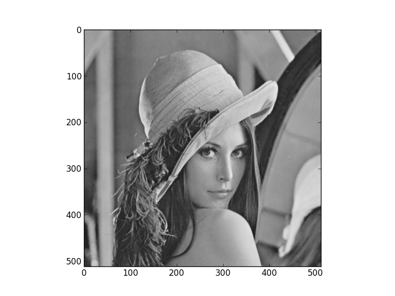
Using the pylab environment (part of matplotlib) we can perform a simple example where we transform the standard ‘Lena’ image and show the level 2 wavelet coefficients:

# Load the Lena image from the Internet into a StringIO object
from StringIO import StringIO
from urllib2 import urlopen
LENA_URL = 'http://www.ece.rice.edu/~wakin/images/lena512.pgm'
lena_file = StringIO(urlopen(LENA_URL).read())

# Parse the lena file and rescale to be in the range (0,1]
from scipy.misc import imread
lena = imread(lena_file) / 255.0

from matplotlib.pyplot import *
import numpy as np

# Show lena on the left
figure(1)
imshow(lena, cmap=cm.gray, clim=(0,1))

import dtcwt

# Compute two levels of dtcwt with the defaul wavelet family
Yh, Yl = dtcwt.dtwavexfm2(lena, 2)

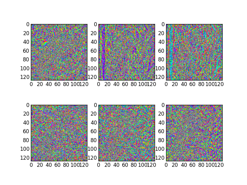
# Show the absolute images for each direction in level 2.
# Note that the 2nd level has index 1 since the 1st has index 0.
figure(2)
for slice_idx in xrange(Yl[1].shape[2]):
    subplot(2, 3, slice_idx)
    imshow(np.abs(Yl[1][:,:,slice_idx]), cmap=cm.spectral, clim=(0, 1))

# Show the phase images for each direction in level 2.
figure(3)
for slice_idx in xrange(Yl[1].shape[2]):
    subplot(2, 3, slice_idx)
    imshow(np.angle(Yl[1][:,:,slice_idx]), cmap=cm.hsv, clim=(-np.pi, np.pi))

show()

If the library is correctly installed and you also have matplotlib installed, you should see these three figures:

3D transform¶

In the examples below I assume you’ve imported pyplot and numpy and, of course, the dtcwt library itself:

import numpy as np
from matplotlib.pyplot import *
from dtcwt import *

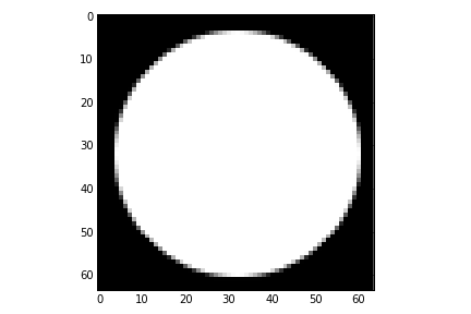
We can demonstrate the 3D transform by generating a 64x64x64 array which contains the image of a sphere:

GRID_SIZE = 64
SPHERE_RAD = int(0.45 * GRID_SIZE) + 0.5

grid = np.arange(-(GRID_SIZE>>1), GRID_SIZE>>1)
X, Y, Z = np.meshgrid(grid, grid, grid)
r = np.sqrt(X*X + Y*Y + Z*Z)

sphere = 0.5 + 0.5 * np.clip(SPHERE_RAD-r, -1, 1)

If we look at the central slice of this image, it looks like a circle:

imshow(sphere[:,:,GRID_SIZE>>1], interpolation='none', cmap=cm.gray)

Performing the 3 level DT-CWT with the defaul wavelet selection is easy:

Yl, Yh = dtwavexfm3(sphere, 3)

The function returns the lowest level low pass image and a tuple of complex subband coefficients:

>>> print(Yl.shape)
(16, 16, 16)
>>> for subbands in Yh:
...     print(subbands.shape)
(32, 32, 32, 28)
(16, 16, 16, 28)
(8, 8, 8, 28)

Performing the inverse transform should result in perfect reconstruction:

>>> Z = dtwaveifm3(Yl, Yh)
>>> print(np.abs(Z - ellipsoid).max()) # Should be < 1e-12
8.881784197e-15

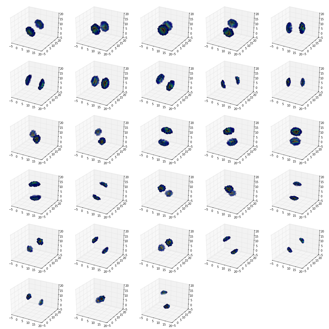
If you plot the locations of the large complex coefficients, you can see the directional sensitivity of the transform:

from mpl_toolkits.mplot3d import Axes3D

figure(figsize=(16,16))
nplts = Yh[-1].shape[3]
nrows = np.ceil(np.sqrt(nplts))
ncols = np.ceil(nplts / nrows)
W = np.max(Yh[-1].shape[:3])
for idx in xrange(Yh[-1].shape[3]):
    C = np.abs(Yh[-1][:,:,:,idx])
    ax = gcf().add_subplot(nrows, ncols, idx+1, projection='3d')
    ax.set_aspect('equal')
    good = C > 0.2*C.max()
    x,y,z = np.nonzero(good)
    ax.scatter(x, y, z, c=C[good].ravel())
    ax.auto_scale_xyz((0,W), (0,W), (0,W))

tight_layout()

For a further directional sensitivity example, see Showing 3D Directional Sensitivity.